Paper Study (Lenet-5)
Study for paper “Gradient Based Learning Applied to Document Recognition”.
Paper
Title: Gradient Based Learning Applied to Document Recognition
Authors: Y. Lecun; L. Bottou; Y. Bengio; P. Haffner
Publisher: IEEE
Published in: Proceedings of the IEEE
Date of Publication: November 1998
IEEE Keywords:
Neural networks, Pattern recognition, Machine learning, Optical character recognition software, Character recognition, Feature extraction, Multi-layer neural network, Optical computing, Hidden Markov models, Principal component analysis
Source Literature: https://ieeexplore.ieee.org/document/726791
Summary
LeNet-5 is a convolutional neural network (CNN) architecture designed for handwritten digit recognition, proposed by Yann LeCun et al. in 1998. It consists of seven layers, including two convolutional layers followed by subsampling layers and three fully connected layers.
LeNet-5, the name is derived from the author LeCun, with ‘5’ being the code for his research accomplishments.
Background
LeNet-5 was developed to address the problem of recognizing handwritten digits in the context of the MNIST dataset, which contains images of handwritten digits ranging from 0 to 9.
LeNet-5 was developed for the purpose of document recognition.
- American Post office Zip Code
- Banking Systems Cheque
Solving the main problem
LeNet-5 tackles the main problem of handwritten digit recognition by utilizing convolutional layers to extract features from the input images and subsampling layers to reduce dimensionality while preserving important features. – efficient , power saving
This hierarchical approach enables the network to learn hierarchical representations of the input data, leading to accurate digit classification. – automatic , higher accuracy for classification
- Handwritten Digit Recognition Need In the early 90s, automated recognition of handwritten digits was crucial for sectors like banking and postal services, but early systems struggled due to reliance on manual feature design and traditional processing techniques.
- Early Neural Network Constraints Limited computational power and lack of data hindered the effectiveness of neural networks in the 90s, affecting their performance and generalization.
- Computer Vision Challenges Before deep learning, computer vision relied on manually designed feature extractors, lacking flexibility and generality for diverse tasks.
Result & Contribution
- Pioneering CNN Application
LeNet-5 introduced Convolutional Neural Networks (CNNs) to handwritten digit recognition, marking the first successful application of CNNs in this field. - Hierarchical Structure Design and Parameter Sharing
LeNet-5 proposed a hierarchical structure with convolutional and pooling layers, along with a parameter sharing mechanism, effectively reducing model parameters and enhancing generalization capability. - Reduced Preprocessing Need
LeNet-5 minimized preprocessing requirements by directly learning features from raw data, simplifying the recognition process for handwritten character recognition. - Introduction of Gradient-Based Learning
LeNet-5 introduced a gradient-based learning neural network structure, enabling automatic feature and pattern learning from data, leading to superior results compared to alternative methods in handwritten character recognition. - Impact on Deep Learning Development
LeNet-5’s successful application significantly influenced the advancement of deep learning, particularly in image recognition, laying the groundwork for subsequent research and applications in the field.
Layers (Key skill)
LeNet-5 consists of a total of 7 layers , trained on grayscale images of size 32 x 32 pixels.
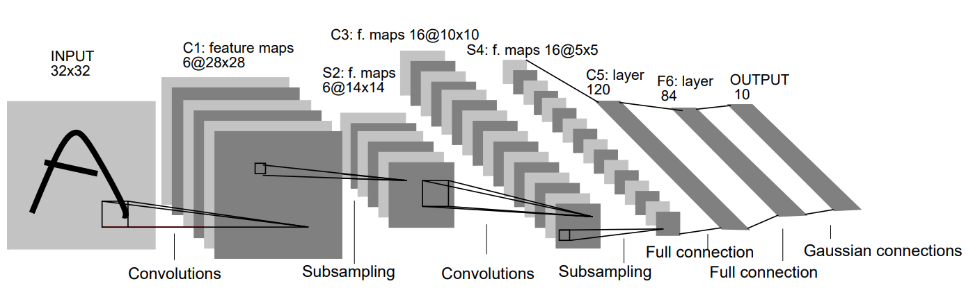
Architecture of LeNet-5
- x — Index of the layer
- Cx — Convolution layer
- Sx — Subsampling layer
- Fx — Fully-connected layer
Key features
- Local Perception
LeNet-5 employs convolutional layers and pooling layers to achieve local perception. By sliding convolutional kernels over the input image, it captures local features, aiding in extracting spatial information from the image. - Weight Sharing
LeNet-5 utilizes weight sharing, where the same convolutional kernel is applied across the entire image. This technique reduces the number of parameters in the network, mitigates overfitting risks, and enhances the model’s generalization ability. - Multiple Convolutional Kernels
Each convolutional layer in LeNet-5 typically consists of multiple convolutional kernels. These kernels learn different features, thereby increasing the network’s ability to represent various aspects of the input image.
A key skill employed by LeNet-5 is convolutional operation, which involves applying filters to the input image to extract features such as edges, corners, and textures. Additionally, LeNet-5 utilizes techniques like subsampling to downsample feature maps, reducing computational complexity while retaining important features.
Note
Output also know as feature map.
Kernel also know as filter
Number of Kernels determine the num of feature map.
Computation of output size :
Input Size: (H,W)
Filter Size: (FH,FW)
Output Size: (OH,OW)
Padding : P
$$ OH = \frac{H + 2 \times P - FH}{S} + 1 $$
$$ OW = \frac{W + 2 \times P - FW}{S} + 1 $$
C1
- Input Size:
32*32 - Kernel Size:
5*5 - Number of Kernels:
6 - Stride:
1 - Output Size:
28*28 - Number of Outputs:
6 - Number of Perceptrons:
6 * 28*28 - Number of Trainable Parameters:
6 * (5*5+1) - Number of Connections:
6 * (5*5+1) * 28 * 28
Different convolutional kernels share the same weights. Thus, when the kernels slide over different positions, they all utilize the same set of weights for feature extraction. This approach reduces the number of parameters in the model while better capturing local features in images.
This is because local features in images typically exhibit translation invariance.
S2
- Input Size:
28*28 - Pooling Window Size:
2*2 - Number of Pooling Window:
6 - Stride:
2 - Output Size:
14*14 - Number of Outputs:
6 - Number of Perceptrons:
6 * 14*14 - Number of Trainable Parameters:
6 * (1+1)(sampling weight + num of bias) - Number of Connections:
6 * (2*2+1) * 14 * 14
Average pooling
Activation Func : Sigmoid
C3
- Input Size:
14*14 - Kernel Size:
5*5 - Number of Kernels:
16 - Stride:
1 - Output Size:
10*10 - Number of Outputs:
16 - Number of Perceptrons:
6 * 14*14 - Number of Trainable Parameters:
6 * (3*(5*5) + 1) + 6*(4*(5*5)+1) + 3*(4*(5*5)+1) + 1*(6*5*5+1) = 1516 - Number of Connections:
10 * 10 * 1516
// table?
S4
- Input Size:
10*10 - Pooling Window Size:
2*2 - Number of Pooling Window:
16 - Stride:
2 - Output Size:
5*5 - Number of Outputs:
16 - Number of Perceptrons:
16 * 5*5 - Number of Trainable Parameters:
16 * (1+1)(sampling weight + num of bias) - Number of Connections:
6 * (2*2+1) * 5 * 5
Average pooling
Activation Func : Sigmoid
C5 (fully-connected layer)
- Input Size:
5*5 - Kernel Size:
5*5 - Number of Kernels:
120 - Stride:
1 - Output Size:
1*1 - Number of Outputs:
120 - Number of Perceptrons:
120 * 1 - Number of Trainable Parameters:
120 * (5*5*16+1) - Number of Connections:
120 * (5*5*16+1) * 1 * 1
channel increase into 16
F6
- Input Size:
1*120 - Output Size:
1*84 - Number of Outputs:
84 - Number of Perceptrons:
84 - Number of Trainable Parameters:
84 * (120 + 1)
Activation Func : Sigmoid
bitmap 7*12
Output (Softmax)
- Input Size:
1*84 - Output Size:
1*10 - Number of Outputs:
10 - Number of Perceptrons:
10 - Number of Trainable Parameters:
10 * (84+1)
RBF
RBF参数的选择确保了F层的sigmoid函数不会饱和,从而使得网络能够在最大的非线性范围内操作,避免了慢收敛和损失函数病态化的问题。
have weight
Gradian Descend
The commonly used loss function in LeNet-5 is the Cross Entropy Loss.
Cross Entropy Loss is a popular loss function used for classification tasks, widely applied in neural networks.
SGD
Adam
Hands-On (pytorch)
Env
Env: Pytorch (docker images pytorch/pytorch:2.1.1-cuda12.1-cudnn8-devel)
Tools: tersorboard
- Container
Base for image
yang_pytorch_env:20240307- pytorch/pytorch:2.1.1-cuda12.1-cudnn8-devel
- Vim
- OpenSSH Server
# Dockerfile FROM yang_pytorch_env:20240307 EXPOSE 8080 22 RUN sed -i 's/#PermitRootLogin prohibit-password/PermitRootLogin yes/' /etc/ssh/sshd_config CMD ["/usr/sbin/sshd", "-D"] - Run Container
docker run -itd --name yang_pytorch_env2 -v /home/ubuntu/yang_pytorch:/workspace -p 0.0.0.0:8080:8080 -p 0.0.0.0:8081:22 --gpus all --ipc=host yang_pytorch_env:20240307_2 /bin/sh -c "while true; do echo hello world; sleep 1; done" - Run Code
python3 lenet5.py - Tensorboard
pip install tensorboard
tensorboard --logdir=runs --port 8080 --bind_all --reload_interval 1.0 --reload_multifile True
Model
Over time and with the advancement of research, various improvements and optimizations have been proposed, primarily focusing on the handling of activation functions and layers in neural networks.
- Activation Functions:
LeNet-5 utilizes Sigmoid and Tanh functions to introduce nonlinearity, whereas modern neural networks more commonly employ ReLU (Rectified Linear Unit) as the activation function. The advantage of ReLU lies in its fast computation speed and avoidance of gradient vanishing issues during backpropagation. - Nonlinearity Placement:
In LeNet-5, nonlinear activation is typically introduced after pooling layers. However, in modern neural networks, activation functions are usually applied immediately after convolutional layers, rather than introducing nonlinearity after pooling layers. This approach is more common as it aligns better with the design principles of neural networks and is easier to train. - Subsampling Strategies in LeNet-5 and CNNs: Average Pooling vs. Max Pooling LeNet-5 and typical CNNs both utilize some form of subsampling layer to reduce the size of feature maps. However, LeNet-5 employs average pooling layers for subsampling, whereas typical CNNs commonly use max pooling layers.
# lenet-5 for training,validating by using gpu
import torch
import torch.nn as nn
import torch.optim as optim
from torchvision import datasets, transforms
from torch.utils.data import DataLoader
from torch.utils.tensorboard import SummaryWriter
import time

# Define the LeNet-5 model
class LeNet5(nn.Module):
    def __init__(self):
        super(LeNet5, self).__init__()
        # Layer C1: Convolutional layer
        self.c1 = nn.Conv2d(in_channels=1, out_channels=6, kernel_size=5, padding=2)
        # Layer S2: Sub-sampling layer -> (Max-Pooling)
        self.s2 = nn.MaxPool2d(kernel_size=2, stride=2)
        # Layer C3: Convolutional layer
        self.c3 = nn.Conv2d(in_channels=6, out_channels=16, kernel_size=5)
        # Layer S4: Sub-sampling layer -> (Max-Pooling)
        self.s4 = nn.MaxPool2d(kernel_size=2, stride=2)
        # Layer C5: Fully connected layer
        self.c5 = nn.Linear(16 * 5 * 5, 120)
        # Layer F6: Fully connected layer
        self.f6 = nn.Linear(120, 84)
        # Output layer
        self.output = nn.Linear(84, 10)

    def forward(self, x):
        # C1 layer
        x = self.c1(x)
        # Sigmoid -> ReLu (After convolution layer)
        x = nn.functional.relu(x)
        # S2 layer
        x = self.s2(x)
        # C3 layer
        x = self.c3(x)
        # Sigmoid -> ReLu (After convolution layer)
        x = nn.functional.relu(x)
        # S4 layer
        x = self.s4(x)
        # Flatten the output for fully connected layers
        x = x.view(-1, 16 * 5 * 5)
        # C5 layer
        x = self.c5(x)
        # Sigmoid -> ReLu
        x = nn.functional.relu(x)
        # F6 layer
        x = self.f6(x)
        x = nn.functional.relu(x)
        # Output layer
        x = self.output(x)
        return x

ROOT_FOLDER_PATH = "./data"
EPOCH = 10
BATCH_SIZE = 64
LR = 0.01

device_name = ""
# Check if CUDA is available
if torch.cuda.is_available() :
    print("GPU is available.")
    device_name = "cuda"
else :
    print("Using CPU.")
    device_name = "cpu"

device = torch.device(device_name)

# Load the dataset
transform = transforms.Compose([
    transforms.ToTensor(),
    transforms.Normalize((0.5,), (0.5,))
])
train_dataset  = datasets.MNIST(root=ROOT_FOLDER_PATH, train=True, transform=transform, download=True)


# Create DataLoader for training, validation, and test sets
train_loader = DataLoader(train_dataset, batch_size=BATCH_SIZE, shuffle=True)

# Split train dataset into train and validation sets
train_size = int(0.8 * len(train_dataset))
val_size = len(train_dataset) - train_size
train_dataset, val_dataset = torch.utils.data.random_split(train_dataset, [train_size, val_size])

# Create DataLoader for training, validation, and test sets
train_loader = DataLoader(train_dataset, batch_size=BATCH_SIZE, shuffle=True)
val_loader = DataLoader(val_dataset, batch_size=BATCH_SIZE, shuffle=False)

# Define the model, loss function, and optimizer
model = LeNet5().to(device)
criterion = nn.CrossEntropyLoss()

# Gradient Descent
optimizer = optim.Adam(model.parameters(), lr=LR)
# Learning rate scheduler
scheduler = optim.lr_scheduler.StepLR(optimizer, step_size=3, gamma=0.1)

# Create a SummaryWriter
writer = SummaryWriter()

total_step = len(train_loader)

start = time.time()

# Train the model
for epoch in range(EPOCH):
    running_loss = 0.0
    total_train_correct = 0
    total_train_samples = 0
    # Train the model
    model.train()

    # Training loop
    for batch_index, (inputs, labels) in enumerate(train_loader):
        inputs, labels = inputs.to(device), labels.to(device)

        # Forward pass
        outputs = model(inputs)
        loss = criterion(outputs, labels)

        # Backward pass
        optimizer.zero_grad()
        loss.backward()
        optimizer.step()

        running_loss += loss.item()

        _, predicted = torch.max(outputs, 1)
        total_train_correct += (predicted == labels).sum().item()
        total_train_samples += labels.size(0)

        if (batch_index+1) % 100 == 0:
            print('[Epoch %d/%d, Batch %d/%d] Train loss: %.3f' % (epoch + 1,EPOCH, batch_index + 1,total_step, running_loss / total_step))
            # Write loss to TensorBoard
            writer.add_scalar('training_loss', running_loss / total_step, epoch * total_step + batch_index)
            running_loss = 0.0

    # Validate the model
    model.eval()
    val_loss = 0.0
    correct = 0
    total = 0
    with torch.no_grad():
        for inputs, labels in val_loader:
            inputs, labels = inputs.to(device), labels.to(device)
            outputs = model(inputs)
            loss = criterion(outputs, labels)
            val_loss += loss.item()
            _, predicted = outputs.max(1)
            total += labels.size(0)
            correct += predicted.eq(labels).sum().item()

    # Adjust learning rate
    scheduler.step()

    # Calculate and print statistics
    train_loss = loss.item()
    train_acc = correct / total
    val_loss /= len(val_loader.dataset)
    print(f"Epoch {epoch + 1}/{EPOCH}, Train Loss: {train_loss:.4f}, Train Acc: {train_acc:.4f}, Val Loss: {val_loss:.4f}")

    # Write accuracy to TensorBoard
    writer.add_scalar('train_accuracy', train_acc, epoch)

end = time.time()
print('Finished Training')
print('Cost time (sec): %d' % (round(end - start, 2)))

# Save the trained model
torch.save(model.state_dict(), "lenet5_mnist_model.pth")

# Close the SummaryWriter after training
writer.close()
# lenet-5 for testing by using gpu
import torch
import torch.nn as nn
import torch.optim as optim
from torchvision import datasets, transforms
from torch.utils.data import DataLoader
from torch.utils.tensorboard import SummaryWriter

# Define the LeNet-5 model
class LeNet5(nn.Module):
    def __init__(self):
        super(LeNet5, self).__init__()
        # Layer C1: Convolutional layer
        self.c1 = nn.Conv2d(in_channels=1, out_channels=6, kernel_size=5, padding=2)
        # Layer S2: Sub-sampling layer -> (Max-Pooling)
        self.s2 = nn.MaxPool2d(kernel_size=2, stride=2)
        # Layer C3: Convolutional layer
        self.c3 = nn.Conv2d(in_channels=6, out_channels=16, kernel_size=5)
        # Layer S4: Sub-sampling layer -> (Max-Pooling)
        self.s4 = nn.MaxPool2d(kernel_size=2, stride=2)
        # Layer C5: Fully connected layer
        self.c5 = nn.Linear(16 * 5 * 5, 120)
        # Layer F6: Fully connected layer
        self.f6 = nn.Linear(120, 84)
        # Output layer
        self.output = nn.Linear(84, 10)

    def forward(self, x):
        # C1 layer
        x = self.c1(x)
        # Sigmoid -> ReLu (After convolution layer)
        x = nn.functional.relu(x)
        # S2 layer
        x = self.s2(x)
        # C3 layer
        x = self.c3(x)
        # Sigmoid -> ReLu (After convolution layer)
        x = nn.functional.relu(x)
        # S4 layer
        x = self.s4(x)
        # Flatten the output for fully connected layers
        x = x.view(-1, 16 * 5 * 5)
        # C5 layer
        x = self.c5(x)
        # Sigmoid -> ReLu
        x = nn.functional.relu(x)
        # F6 layer
        x = self.f6(x)
        x = nn.functional.relu(x)
        # Output layer
        x = self.output(x)
        return x

ROOT_FOLDER_PATH = "./data"
BATCH_SIZE = 64

# Load the dataset
transform = transforms.Compose([
    transforms.ToTensor(),
    transforms.Normalize((0.5,), (0.5,))
])
test_dataset = datasets.MNIST(root=ROOT_FOLDER_PATH, train=False, transform=transform, download=True)
test_loader = DataLoader(test_dataset, batch_size=BATCH_SIZE, shuffle=False)

print(test_dataset.data.size())
print(test_dataset.targets.size())

device_name = ""
# Check if CUDA is available
if torch.cuda.is_available() :
    print("GPU is available.")
    device_name = "cuda"
else :
    print("Using CPU.")
    device_name = "cpu"

device = torch.device(device_name)

model = LeNet5().to(device)
# Testing
# Load the model weights
model.load_state_dict(torch.load('lenet5_mnist_model.pth'))
model.eval()  # Set model to evaluation mode

total_test_correct = 0
total_test_samples = 0

with torch.no_grad():
    for batch_index,(inputs, labels) in enumerate(test_loader):
        inputs, labels = inputs.to(device), labels.to(device)
        outputs = model(inputs)
        _, predicted = torch.max(outputs.data, 1)
        total_test_correct += (predicted == labels).sum().item()
        total_test_samples += labels.size(0)

print(f'Test Accuracy: {100 * total_test_correct / total_test_samples}%')
Check gpu support
device = torch.device("cuda" if torch.cuda.is_available() else "cpu")
# Define the model, loss function, and optimizer (gpu)
model = LeNet5().to(device)
# Move inputs and labels to GPU
inputs, labels = inputs.to(device), labels.to(device)
Check container memory
docker stats
References
https://pytorch.org/vision/main/generated/torchvision.datasets.MNIST.html
https://pytorch.org/docs/stable/generated/torch.nn.Conv2d.html
https://pytorch.org/docs/stable/generated/torch.optim.SGD.html
https://pytorch.org/docs/stable/generated/torch.Tensor.view.html
https://pytorch.org/docs/stable/generated/torch.no_grad.html
https://pytorch.org/docs/stable/data.html#torch.utils.data.random_split
https://pytorch.org/docs/stable/tensorboard.html